Generate Cycle-Specific Plots and Summary Data for a Given ID — cycle_plot

This function creates cycle-specific plots and summary statistics for a specified individual (id), storing both in a named list for easy access.

Usage

cycle_plot_individual(
  data,
  id,
  symptoms,
  centering = "menses",
  y_scale = "person-centered",
  include_impute = TRUE,
  rollingavg = 5
)

Arguments

data: A dataframe containing menstrual cycle data, including id and cyclenum columns.
id: Numeric id number for the specific individual for whom cycle plots should be generated.
symptoms: A vector of strings specifying the symptom variable to analyze that exist in data.
centering: A string indicating the centering phase of the cycle ("menses" or "ovulation").
y_scale: A string specifying the y-axis scale ("person-centered", "person-centered_roll", "raw", or "roll").
include_impute: A boolean indicating whether to use imputed cycle time values.
rollingavg: A numeric indicating how many days of a rolling average to use, the default is 5

Value

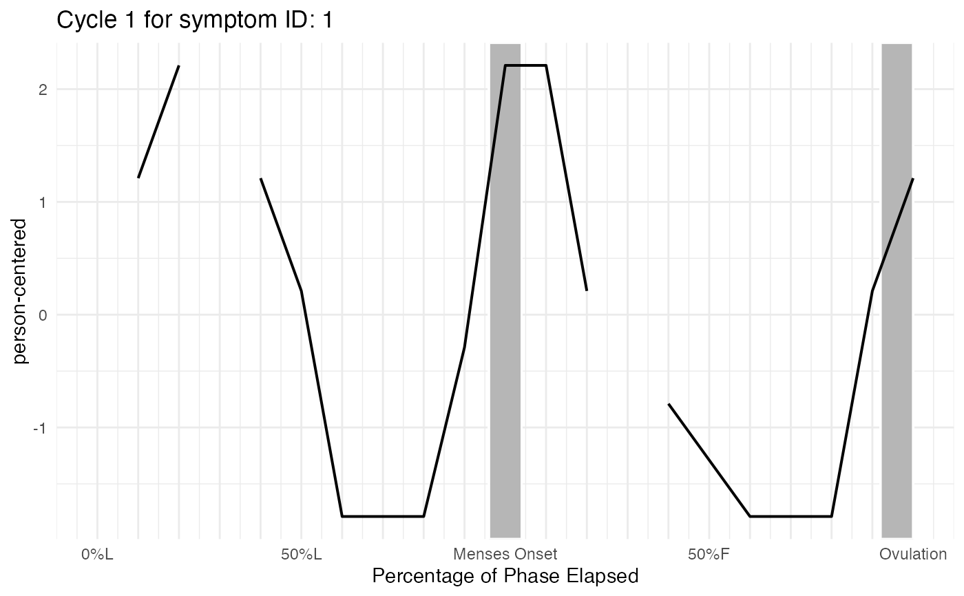
A named list, one element per entry in symptoms. Each of those is itself a named list, one element per cycle (named "Cycle_1", "Cycle_2", ...), each containing:

$plot: The cycle-specific ggplot object with the ID displayed
$summary: The corresponding summary data

So for a single symptom "symptom" and its first cycle, access the plot as result[["symptom"]][["Cycle_1"]]$plot.

Examples

cycle_df = cycledata

data_with_scaling <- pacts_scaling(
  cycle_df,
  id = id,
  date = daterated,
  menses = menses,
  ovtoday = ovtoday,
  lower_cyclength_bound = 21,
  upper_cyclength_bound = 35
)

result <- cycle_plot_individual(
  data_with_scaling,
  id = unique(data_with_scaling$id)[1],
  symptoms = "symptom"
)

# the first cycle's plot and summary for "symptom":
result[["symptom"]][["Cycle_1"]]$plot
#> Warning: Removed 1 row containing missing values or values outside the scale range
#> (`geom_line()`).

result[["symptom"]][["Cycle_1"]]$summary
#> # A tibble: 20 × 7
#>    cycleday_5perc mean_dev mean_dev_roll raw_sx sx_roll cycleday mcyclength
#>             <dbl>    <dbl>         <dbl>  <dbl>   <dbl>    <dbl>      <dbl>
#>  1           0     NaN            0.877   NaN      3.67     11           24
#>  2           0.05    1.21         1.63      4      4.42     12.5         24
#>  3           0.1     2.21         1.88      5      4.67     14           24
#>  4           0.15  NaN            1.46    NaN      4.25     15           24
#>  5           0.2     1.21         1.04      4      3.83     16.5         24
#>  6           0.25    0.211        0.211     3      3        18           24
#>  7           0.3    -1.79        -1.04      1      1.75     19.5         24
#>  8           0.35   -1.79        -1.54      1      1.25     21           24
#>  9           0.4    -1.79        -1.19      1      1.6      22           24
#> 10           0.45   -0.289       -0.914     2.5    1.88     23.5         24
#> 11           0.5     2.21         1.54      5      4.33      1           24
#> 12           0.55    2.21         1.54      5      4.33      2           24
#> 13           0.6     0.211        0.961     3      3.75      3           24
#> 14           0.65  NaN           -0.0395  NaN      2.75      4           24
#> 15           0.7    -0.789       -1.04      2      1.75      5           24
#> 16           0.8    -1.79        -1.54      1      1.25      6           24
#> 17           0.85   -1.79        -1.19      1      1.6       7           24
#> 18           0.9    -1.79        -0.789     1      2         8           24
#> 19           0.95    0.211       -0.539     3      2.25      9           24
#> 20           1       1.21        -0.123     4      2.67     10           24